Detecting the magnetopause

Understanding the shape and location of the magnetopause is crucial to explaining the dynamics and processes of geophysical plasmas, and particularly the response of the magnetosphere to the solar wind. How does the subsolar point change with the dynamic and magnetic pressure of the solar wind? How does the IMF affect the position of the cusps, and what can this indicate for the magnetic reconnection that takes place to form them? With which processes can this collisionless plasma interact with obstacles and display fluid like behavior?

In-situ satellite measurements

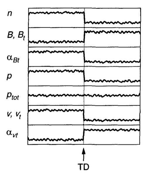
Fig. 5 Typical behavior of plasma moments along a tangential discontinuity [Baumjohann and Treumann, 2006].

We have partial answers to these questions through in-situ measurements of satellite crossings. By analyzing the measurements of instruments on board and detecting abrupt changes in parameters such as density, temperature, flow velocity, and magnetic field orientation, we can identify the location and type of discontinuity and correlate it with the position of the satellite. A typical magnetopause crossing from the Cluster 1 spacecraft is shown in Fig. 6.

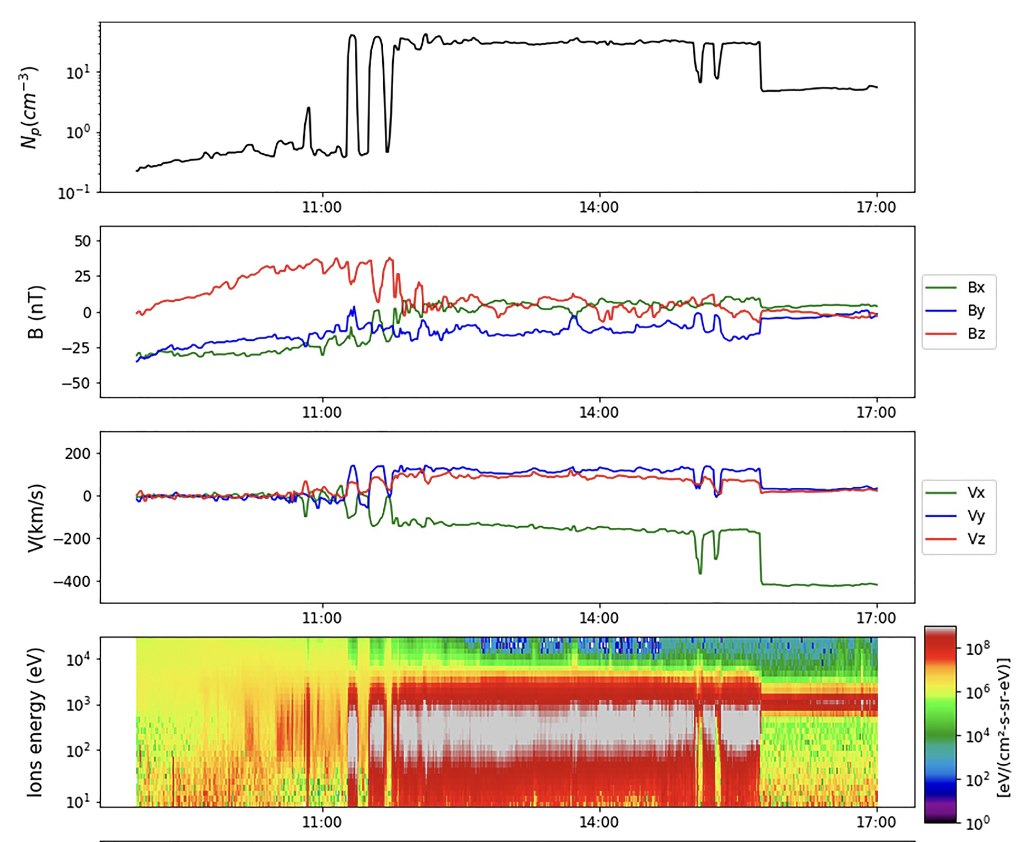
Fig. 6 Cluster 1 spacecraft measurements while crossing from the solar wind to the magnetosheath to the magnetosphere [Nguyen et al., 2022].

In order to derive information about the global behavior of this surface, one must compile a catalog of boundary crossings from multiple in situ data of such missions. This quite a time-consuming task, as well as ambiguous concerning the interpretation of the measurements and the precise definition and automatic detection of the crossings. The ever-growing amount of data collected by the satellites, therefore does not linearly translate to increasing number of catalogs [Nguyen et al., 2022]. Additionally, the dynamic nature of the response of the magnetopause to the solar wind, make the correlation of local measurements, with the global shape and dynamics of the magnetopause challenging. Nonetheless, various studies have attempted characterizing and parametrizing this shape with \ac{SW} and magnetospheric parameters, building thus empirical models of the surface.

Coordinate system

Before moving any further, we shall define our main coordinate systems and frames, for consistency. The most common frame we will be using is the Geocentric Solar Ecliptic (GSE) system. This has its X-axis pointing from the Earth toward the Sun and its Y-axis is chosen to be in the ecliptic plane pointing towards dusk (thus opposing planetary motion). Its Z-axis is parallel to the ecliptic pole. Relative to an inertial system this system has a yearly rotation.

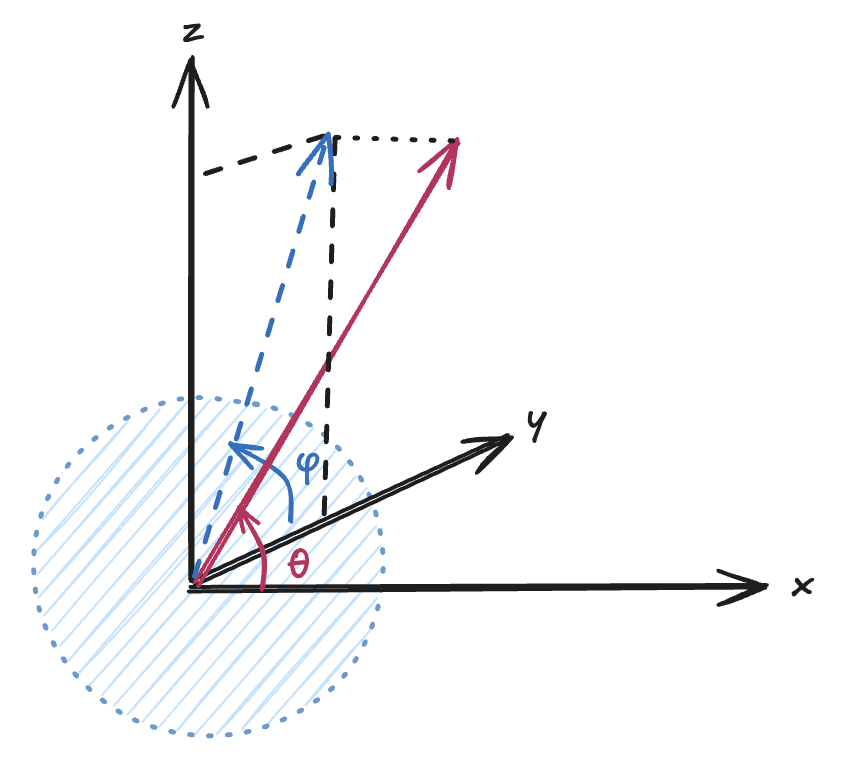
Fig. 7 GSE and spherical coordinates.

\[x = r cos\theta\]

\[ y = r sin\theta cos \phi\]

\[z = r sin\theta sin\phi \]

We can define a spherical system based on the cartesian GSE, that will help us describe the magnetopause as a parametrized radial function of the spherical angles \(r(\theta,\phi)\). We follow the convention of previous papers [Sun et al., 2020], where \(\theta\) is the angle between \(\vec{r}\) and the X-axis, and \(\phi\) is the angle between the Y-axis and the projection of \(\vec{r}\) to the YZ plane. The coordinate transformation from spherical to GSE is therefore defined as in Fig. 7.

Empirical models

Moving back to the study of the magnetopause surface through the statistical analysis of crossings, we will look into the main empirical models that have been proposed. The first and simplest empirical model was proposed by [Shue et al., 1997] and is described by Equation (2).

(2)\[ r(\theta) = r_0 \left( \frac{2}{1 + \cos \theta} \right)^\alpha \]

where:

\(r(\theta)\)

Radial distance of the magnetopause from the Earth’s center at a given polar angle \(\theta\)

\(\text{R}_E\)

Earth’s radius (~6371 km)

\(\alpha\)

the flaring parameter, given by: \(\alpha = (0.58 - 0.01 B_z) (1 + 0.01 P_{dyn})\)

\(P_{dyn}\)

Dynamic pressure of the solar wind (in nPa): \(P_{dyn} = 1.15 \cdot n \cdot v_x^2 \cdot 1.67 \times 10^{-6}\)

\(r_0\)

Subsolar standoff distance of the magnetopause,given by: \(r_0 = (11.4 + 0.013 B_z) P_{dyn}^{-\frac{1}{6.6}}, \quad \text{for } B_z \geq 0\) \(r_0 = (11.4 + 0.14 B_z) P_{dyn}^{-\frac{1}{6.6}}, \quad \text{for } B_z < 0\)

Here, the relations that are given for \(\alpha\) and \(r_0\) are the parametrization with respect to the solar wind and magnetospheric parameters, derived in the original paper [Shue et al., 1997]. The crossings used to construct this model where taken from satellites of equatorial orbit, and thus assumes a rotational symmetry over the X-axis. As expected from the numerical solution of the surface in the equatorial plane, no discontinuity arises, and therefore the Shue model describes a smooth surface with no indentations.

Later evidence of dipole tilt, indentation in the near-cusp region, and dawn-dusk asymmetry led to the development of more refined models. One such improvement was introduced by [Lin et al., 2010], who proposed an empirical magnetopause model that included an azimuthal asymmetry induced by the dipole tilt angle and also kept the possibility of a dawn-dusk asymmetry [Lin et al., 2010]. In his paper [Liu et al., 2015] combined THEMIS data and MHD simulations to derive a more sophisticated geometry and parametrization \cite{liu}. We will describe these models concisely, as expressed by [Nguyen et al., 2022, Nguyen et al., 2022], where he defines the general form Equation (3).

(3)\[ r = r_0 \left( \frac{2}{1 + \cos\theta} \right)^{\xi} + Q \]

where, Q is an additive term that defines the geometry of the cusps, and is different for the two models. For the Lin model, this term is expressed by:

\[\begin{split} &Q = C \left( e^{d_n \psi_n^{4/5}} + e^{d_s \psi_s^{4/5}} \right) \\ &C = a_9 (P_{dyn} + P_n)^{a_{10}} \\ &d_{n,s} = a_{11} \pm a_{12} \gamma + a_{13} \gamma^2 \\ &\psi_n = \arccos\left( \cos(\theta) \cos(\theta_n) + \sin(\theta) \sin(\theta_n) \cos(\phi) \right) \\ &\psi_s = \arccos\left( \cos(\theta) \cos(\theta_s) + \sin(\theta) \sin(\theta_s) \cos(\phi - \pi) \right) \\ &\theta_{n,s} = a_{14} \pm a_{15} \gamma \end{split}\]

The terms \(\psi_n\) and \(\psi_s\) describe the angular distance from the cusp indentations in the northern and southern hemispheres, respectively. The additive term of the Liu model is described by the following equations:

\[\begin{split} &Q = -a_9 C r_0 \left( \frac{2}{1 + \cos\theta} \right)^{\xi} \cos^2\phi\\ &C = e^{-|\theta - l_n|/w} \left( 1 + \text{sgn}(\cos\phi) \right) + e^{-|\theta - l_s|/w} \left( 1 + \text{sgn}(\cos(-\phi)) \right) \\ &l_{n,s} = \left( a_{10} + a_{11} \tanh[a_{12}(B_z + a_{13})] \right) (1 \mp a_{14} \gamma) \\ &w = \left( a_{15} + a_{16} \log(P_{dyn}) \right) (1 + a_{17} \gamma^2) \end{split}\]

We advise the reader to refer to the corresponding studies for more information on the coefficients \(a_i\) and the way they are determined\cite{nguyen4}. In his paper series, [Nguyen et al., 2022], re-parametrizes and evaluates this models by analyzing multi-mission data and constructing a representative catalog. Among the many relevant results, is that the Lin model overestimates the indentation of the cusps, while the Liu model seems to be the best description of the selected crossings. We will see later on, that this comes in disagreement with some of our results, depending on how we define the magnetopause, and extra care must be taken to ensure consistent definitions.

Imaging the magnetopause

It is evident that we have gained valuable knowledge from these in-situ measurements, however the global dynamics of the magnetopause and its response to the solar wind are still difficult to extract. The capability of remote sensing, or imaging of this boundary, would allow for more dynamic measurements; something that is crucial for understanding the coupling with the solar wind, which can be highly variable in a timescale of minutes. Under this scope, it was proposed that we could utilize the charge exchange phenomenon between the solar wind and the exosphere of the Earth, to achieve this new method of observation.

Charge exchange

The geocorona is the outermost region of the Earth’s atmosphere, the exosphere, where collisions between particles are considered negligible. The density in this region is generally assumed to drop as \(n_H = 25(\frac{10RE}{R})^3 [cm^{-3}]\)}

During its close approach to Earth, extreme ultraviolet and X-ray emission was observed from the comet C/Hyakutake 1996 B2 by the Röntgen X-ray Satellite and Rossi X-ray Timing Explorer [Lisse et al., 1996]. This emission was later interpreted by [Cravens, 1997] and the charge exchange emission mechanism was proposed. Under this mechanism, the multiply charged heavy ions of the solar wind can charge transfer with cometary neutrals, producing ions which can be highly excited and consequently emit photons in the extreme ultraviolet and x-ray part of the spectrum [Cravens, 1997]. It was later suggested, that the same phenomenon could take place between the solar wind and the geocoronal hydrogen, leading to the terrestrial magnetosheath being luminous in the X-ray regime [Robertson and Cravens, 2003]. The emission in this case, is generated by charge exchange reactions between multiply charged heavy solar wind ions \((\text{O}^{7+}, \text{C}^{5+},\dots)\) and the neutral particles (mostly hydrogen atoms) in the geocorona. The general SWCX interaction is given by Equation (4).

(4)\[ \text{X}^{q+} + \text{M} \rightarrow \text{X}^{(q-1)+*} + \text{M}^+, \]

where the heavy and multiply charged \((q+)\) solar wind ion is noted as \( \text{X}^{q+}\) and the neutral particle is noted as \(\text{M}\). Electrons are transferred from neutral particles to a high energy state of ions, imposing these ions into an excited state. When the excited ions de-excite to the lower-energy state, they emit photons in the soft X-ray band \((E \leq 2 keV)\) [Xu et al., 2024]:

\[ \text{X}^{(q-1)+*} \rightarrow \text{X}^{(q-1)+} + h\nu \]

In their paper, [Robertson and Cravens, 2003], simulated this emission as images, opening the discussion about remote sensing of the magnetosheath. Soft X-ray emissivity is expected to be strong in the dayside magnetosheath and cusp regions, where both solar wind ion and neutral particle densities are high. In contrast, the low density of solar wind ions within the magnetosphere and the scarcity of neutral hydrogen in the solar wind result in weak emission in those regions. As a result, a boundary in soft X-ray emission is expected at the magnetopause. This sharp increase in emission can be used to determine the magnetopause location through global soft X-ray imaging from space-based instruments. [Sibeck et al., 2018]

SMILE mission

The SMILE mission was proposed, in collaboration of \European Space Agency (ESA) and Chinese Academy of Sciences (CAS), as an attempt in capturing this Solar Wind Charge Exchange (SWCX) phenomenon in the Earth’s magnetosheath. The satellite will be launched in 2026 into a highly elliptical polar orbit, with an apogee of \(\approx 20\) Earth Radii (RE), a perigee of \(\approx 1\) RE, and an inclination of \(73^\circ\). The orbital period is \(\approx 50.3\) hours, and a schematic of its orbit is shown in \autoref{fig:orbit}. The science payload on-board SMILE consists of the UltraViolet Imager (UVI), the MAGnetometer (MAG), the Light Ion Analyser (LIA) and finally the Soft X-ray Imager (SXI). SXI is a wide FOV X-ray telescope of \(15.5^\circ \times 26.5^\circ\), designed to capture the emission of the magnetosheath, allowing the study of the magnetopause dynamics and its detection with a requirement of \(0.5\,RE\) accuracy. [Sembay et al., 2024]

The preparation for space observations that haven’t been performed before is no trivial task. Space missions require meticulous planning and therefore accurate predictions of the expected science data, as well as methods to optimize their return. The deployment of sophisticated simulations is therefore crucial prior to mission launch, both to facilitate operation planning and to develop pipelines for the analysis of the upcoming data. In this light, the SMILE Modeling Working Group was formed, in order to produce a simulation catalog for different SW conditions, with common input parameters.

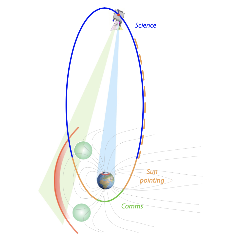
Fig. 8 The SMILE orbit. SXI and UVI Field of View and key regions, credit: ESA

The group aims to predict and interpret the images the SXI will generate, simulate the changes of magnetospheric boundary locations under different solar wind conditions, and extract magnetospheric boundary and cusp positions. To achieve these goals, the Modeling Working Group primarily relies on MHD simulations, which treat the plasma as a single fluid and are computationally efficient. MHD is well-suited for capturing large-scale dynamics and global structures - even in highly dynamic cases, but it lacks kinetic resolution and cannot distinguish between different ion species. As a result, MHD-based X-ray simulations tend to produce smooth, continuous images where the X-ray intensity is strictly proportional to the total proton flux. This leads to two key limitations: the inability to resolve spectroscopic features linked to specific ions, and the artificial production of X-rays within the magnetosphere due to the absence of a distinction between solar wind and magnetospheric plasma. The latter requires the introduction of an artificial mask inside the magnetosphere.

To address these issues, the LATMOS team developed the LATMOS Test Particle (LaTeP) model, a test-particle model that simulates heavy ions kinetically. This intermediate approach introduces ion-specific behavior such as gyroradius effects and charge-exchange cross-section differences, enabling more realistic X-ray spectroscopic predictions and avoiding emission inside the magnetosphere. Since LaTeP does not compute E/B fields self-consistently, it relies on external electromagnetic field inputs provided by MHD codes such as OpenGGCM, justified by the negligible feedback of highly charged ions due to their very low abundance (\(10^{-4}\) the proton density) in the solar wind. Through this approach, we can get the X-ray emissivity by following numerical test-particles, representing heavy ions. In this work we will focus on \(O^{7+}\) ions, since they are the most important contributors in the spectral energy range of the SXI detectors. Solving their equation of motion as they propagate in the MHD-computed \(E\) and \(B\) fields, we calculate the probability of them charge exchanging with hydrogen atoms from the Earth’s exosphere. From this quantity, we can calculate the volume emissivity of X-ray \(Q\) in \(eV\, cm^{-3}\, s^{-1}\), as in (5). [Xu et al., 2024]

(5)\[ Q = n_M \cdot n_{\text{X}^{q+}} \cdot v_{\text{X}^{q+}} \cdot \sigma_{\text{X}^{q+},M} \cdot Y_{\text{X}^{(q-1)+}} \]

where:

\(Q\)

Volume emissivity of soft X-rays (in eV cm\(^{-3}\) s\(^{-1}\))

\(n_M\)

Neutral particle density (cm\(^{-3}\))

\(n_{\text{X}^{q+}}\)

Density of solar wind ions with charge \(q+\) (cm\(^{-3}\))

\(v_{\text{X}^{q+}}\)

Plasma (ion) velocity (cm s\(^{-1}\))

\(\sigma_{\text{X}^{q+},M}\)

Cross-section for charge exchange between \(\text{X}^{q+}\) and \(M\) (cm\(^2\))

\(Y_{\text{X}^{(q-1)+}}\)

Energy of emitted line weighted by its emission probability (eV)

We can integrate this emissivity along a specific Line Of Sight (LOS) to obtain the intensity of each looking direction in \(eV cm^{-2} s^{-1} sr^{-1}\). We also assume isotropic emission and divide by \(4\pi\) to get the emissivity in a particular direction.

\[ I = \frac{1}{4\pi} \int_{LOS} Q\,ds \]

Calculating this quantity for each pixel’s LOS of the imager, we can construct a synthetic image of the expected SXI data. This does not take into account the contribution from background sources nor the response of the instrument.