Introduction

Although the matter we encounter daily on Earth’s surface predominantly exists in solid, liquid, or gaseous states, the vast majority of baryonic matter in the universe exists in a fourth state: plasma. This state of matter displays complex behaviors that have not been completely understood due to the lack of proximity to naturally occurring plasmas as well as their vast diversity in density and temperature. The closest natural laboratory to study these plasmas is the Earth itself, particularly in the region above approximately 100 km altitude, where the phenomena that take place are dominated by electromagnetic interactions and should be treated using plasma physical methods. A key point of interest is the interaction and coupling of the Sun - Earth system, also known as space weather. We will attempt to study this connection and the physics between the interaction of the Sun’s emitted particles and the terrestrial space environment.

Earth’s Space Environment

We characterize this region as the Earth’s space environment, consisting of the magnetosphere and its neighboring plasma regions, that display strong coupling, as well as a plethora of different phenomena. To understand this environment we shall start from its driving forces:

The Sun emits magnetized supersonic plasma with typical speeds of 300 to 800 km/s. This is known as the Solar Wind (SW), consisting mainly of electrons, protons and alpha particles, as well as traces of atomic nuclei and heavy ions found in the solar corona, such as carbon, nitrogen, oxygen, neon, magnesium, silicon, sulfur, and iron. The solar wind plasma is highly conductive meaning the magnetic field lines and the plasma flows are “frozen” together and the coronal magnetic field is dragged out by the solar wind to form the Interplanetary Magnetic Field (IMF).

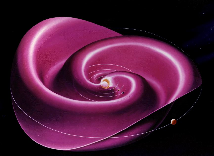
Fig. 1 Parker spiral of Interplanetary Magnetic Field

This takes the shape of an Archimedean spiral pattern due the combination of the outward motion of the solar wind and the Sun’s rotation, known as the Parker spiral [Parker, 1958] and shown schematically in Fig. 1. Near the Earth, the IMF can be expressed as a three-dimensional vector \(\vec{B} = B_x \vec{x}+B_y \vec{y}+B_z \vec{z}\). Its coupling to the Earth’s magnetic field is correlated with its local orientation. We can parametrize this through the ‘clock angle’ \(\Omega\), which describes the orientation of the magnetic field in the Y-Z plane of the Geocentric Solar Magnetospheric (GSM) coordinate system. A clock angle of \(0^\circ\) means the IMF points northward, parallel to Earth’s magnetic dipole, while a clock angle of \(180^\circ\) means the IMF points southward.

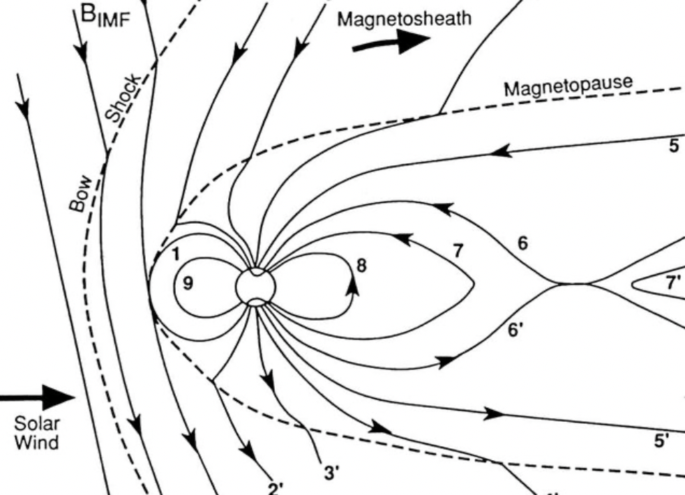
Fig. 2 Plasma regions of the near-Earth environment

The Earth generates its own magnetic field as well, owing its existence to the currents induced by the convective motion in its core. Due to its supersonic velocity, when the solar wind encounters an obstacle, like the Earth’s magnetic field, it is decelerated and deflected, forming a bow shock where the kinetic energy of the supersonic plasma is partially converted to thermal energy. Shocks are discontinuities that are characterized by non-vanishing normal fluxes \(n v_n \neq 0\), meaning the solar wind plasma can penetrate further towards the Earth. The region downstream of the bow shock, called the magnetosheath, contains this thermalized and dense plasma with a stronger magnetic field compared to the undisturbed solar wind. [Baumjohann and Treumann, 2006]

The frozen-in interplanetary magnetic field lines prevent penetration of the solar wind into the magnetosphere, the region where the magnetic field lines of the Earth dominate. The boundary separating these regions is the magnetopause, enclosing the magnetosphere—the cavity formed by the terrestrial magnetic field, compressed on the day-side and elongated into a magnetotail on the night-side by solar wind pressure.