Radial extraction of full magnetopause

Extracting the zero contours through the contour maps of each slice would be a tedious task. To obtain the full surface information we can instead transfer the emissivity cube from the GSE to spherical coordinates in order to treat each radial direction separately. A script for this transformation was provided by Samuel Wharton (SXI team, University of Leicester) and is part of his work on the CMEM model [Wharton et al., 2025].

We can call it as a method of the cube object:

R, Theta, Phi, Q_sph = cube.cartesian_to_spherical(rmax = 15, dtheta = 0.5, dphi = 0.5)

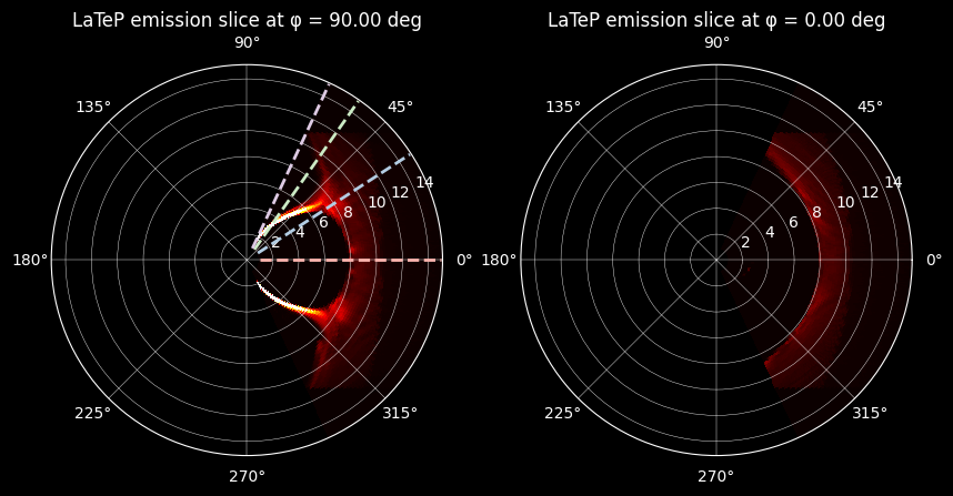
The result is the same emissivity cube, but instead of 3D array representing each dimension of the box (x, y, z) we have discretized \(\phi\in[0,360]^o\) and \(\theta\in[-65,65]^o\) with a step of \(0.5^o\) and \(r\in[0,15]\,RE\) with a step of \(0.2\,RE\). We did not let \(\theta\) range all the way to \(\pi/2\) since there is no physical information from the simulation box in that region. Here the spherical slices corresponding to the GSE \(y=0\) and \(z=0\) cuts:

Show code cell source Hide code cell source

fig, axs = plt.subplots(1, 2, figsize=(10, 5), subplot_kw={'projection': 'polar'})

phi_index = 180
axs[0].pcolormesh(Theta[:, :, phi_index], R[:, :, phi_index], Q_sph[:,:,phi_index], cmap='hot',vmax=1e-4)
theta_lines = [0, np.deg2rad(33), np.deg2rad(55), np.deg2rad(65)]
c = 0
for t in theta_lines:
    axs[0].plot([t, t], [R[:, :, phi_index].min(), R[:, :, phi_index].max()], color=cmap(c), linestyle='--', linewidth=2)
    c+=1
axs[0].set_title("LaTeP emission slice at φ = {:.2f} deg".format(np.degrees(Phi[0, 0, phi_index])))
axs[0].grid(which='major', color='white', linewidth=0.3)

phi_index = 0
axs[1].pcolormesh(Theta[:, :, phi_index], R[:, :, phi_index], Q_sph[:,:,phi_index], cmap='hot',vmax=1e-4)
axs[1].set_title("LaTeP emission slice at φ = {:.2f} deg".format(np.degrees(Phi[0, 0, phi_index])))
axs[1].grid(which='major', color='white', linewidth=0.3)


plt.show()

To better understand the radial profile of the volume emissivity, we plot it versus the radius for different polar \(\theta\) directions:

The \(\phi=90^o\) plane was chosen since it is the one displaying more complex behavior due to the cusps. The typical behavior near the subsolar point is shown in below, where a steep increase appears at the edge of the magnetosphere, forming a global maximum in the X-ray emissivity. In the first figure the same directions are plotted, along with \(\theta=54^o\) which crosses the polar cusp. We can see that the emissivity of this region is significantly prominent, overshadowing the second peak that appears close to the outer boundary of the magnetosphere.

Show code cell source Hide code cell source

fig, axs = plt.subplots(1, 2, figsize=(12, 4))

ph = 180
th = 180
axs[0].plot(R[th,10:,ph],Q_sph[th,10:,ph], label= f"θ = {np.degrees(Theta[th, 0, ph]):.2f} deg", color=cmap(0))
th = -90
axs[0].plot(R[th,10:,ph],Q_sph[th,10:,ph], label= f"θ = {np.degrees(Theta[th, 0, ph]):.2f} deg", color=cmap(1))
th = -1
axs[0].plot(R[th,10:,ph],Q_sph[th,10:,ph], label= f"θ = {np.degrees(Theta[th, 0, ph]):.2f} deg", color=cmap(3))
th = -30
axs[0].plot(R[th,10:,ph],Q_sph[th,10:,ph], label= f"θ = {np.degrees(Theta[th, 0, ph]):.2f} deg", color=cmap(2))
axs[0].set_title(f"Cusp radial profile at φ = {np.degrees(Phi[th, 0, ph]):.2f} deg")
axs[0].set_xlabel("R [RE]")
axs[0].set_ylabel("Emissivity [$eV/cm^3/s/sr$]")
axs[0].legend()

th = 180
axs[1].plot(R[th,10:,ph],Q_sph[th,10:,ph], label= f"θ = {np.degrees(Theta[th, 0, ph]):.2f} deg", color=cmap(0))
th = -90
axs[1].plot(R[th,10:,ph],Q_sph[th,10:,ph], label= f"θ = {np.degrees(Theta[th, 0, ph]):.2f} deg", color=cmap(1))
th = -1
axs[1].plot(R[th,10:,ph],Q_sph[th,10:,ph], label= f"θ = {np.degrees(Theta[th, 0, ph]):.2f} deg", color=cmap(3))
axs[1].set_title(f"Radial profiles at φ = {np.degrees(Phi[th, 0, ph]):.2f} deg")
axs[1].set_xlabel("R [RE]")
axs[1].set_ylabel("Emissivity [$eV/cm^3/s/sr$]")
axs[1].legend()

plt.show()

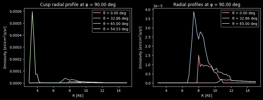
In previous work, various diagnostics of this curve have been used to define the magnetopause surface, such as the global maximum [Sun et al., 2020], the maximum gradient [Samsonov et al., 2022], as well as the quarter of the distance between the maximum gradient and the global maximum [Read, 2024]. The shape of the magnetopause is not significantly affected by this choice. Since our goal in this section is to eventually test the tangent hypothesis, the maximum emissivity is a more suitable metric to compare to the integrated maximum intensity curve.

We can find the indexes of the maximum emissivity of each radial direction and plot them both as slices and as a 3D surface using plotly.graph_objects. It is evident that a lot of information is being obscured by the cusp’s maxima and their inward curvature. The peaks characterizing the outer boundary of the magnetosphere are not registered, as the cusps act as a “wall” for those radial directions.

To bypass this problem, we tried to utilize the difference of magnitude of the emissivity in the cusps and the outer boundary, by finding all the peaks of the radial emissivity and keeping only those that are below an arbitrary threshold of \(1e-5eV/cm^3/s/sr\). This improves the results to some extent, but is not a robust enough definition to result in a continuous and coherent surface.

Finally, we also tried setting a lower limit to the radius of the maximum, to avoid some jumps to very low altitudes, which were mostly the result of simulation discontinuities.

You can change the values threshold and r_skip in the notebook, to see the resulting surface for each case. You can also comment out the uniform_filter(r_surface, size=7) to test what happens if we smooth the surface.

# Choose a threshold value for the maximum intensity and the minimum radius 
threshold = 8e-5 # maximum intensity of peak 
r_skip = 30 # minimum radius in indexes

print(f"Discarding radius below {R[0, r_skip, 0]} Re and Emissivity above {threshold}")

ind_max_below_thresh = np.full((Q_sph.shape[0], Q_sph.shape[2]), -1, dtype=int)

# Loop over theta and phi
for i_theta in range(Q_sph.shape[0]):
    for i_phi in range(Q_sph.shape[2]):
        profile = Q_sph[i_theta, r_skip:, i_phi]  # profile along r
        
        # Find local maxima
        peaks, _ = find_peaks(profile)
        
        # Filter by threshold
        peaks_below = peaks[profile[peaks] < threshold]
        
        if len(peaks_below) > 0:
            # Choose the maximum among the low ones
            best_peak = peaks_below[np.argmax(profile[peaks_below])]
            ind_max_below_thresh[i_theta, i_phi] = best_peak+r_skip

Discarding radius below 7.0 Re and Emissivity above 8e-05

Show code cell source Hide code cell source

# Generate the surface r(theta, phi) and corresponding theta and phi
r_surface = R[np.arange(R.shape[0])[:, None], ind_max_below_thresh, np.arange(R.shape[2])]
theta_surface = Theta[:, 0, 0]
phi_surface = Phi[0, 0, :]

# # Apply 2D moving average with a window size (e.g., 5x5)
# r_surface = uniform_filter(r_surface, size=7)

# Create a grid for the surface plot
theta_grid, phi_grid = np.meshgrid(theta_surface, phi_surface, indexing='ij')

# Convert spherical to Cartesian coordinates for surface plotting
x = r_surface* np.cos(theta_grid) 
y = r_surface * np.sin(theta_grid) * np.cos(phi_grid)
z = r_surface * np.sin(theta_grid) * np.sin(phi_grid)
# Create the interactive 3D surface plot
fig = go.Figure(data=[go.Surface(
    x=x,
    y=y,
    z=z,
    surfacecolor=r_surface,
    colorscale='thermal',
    cmin=0,
    cmax=np.nanmax(r_surface),
    colorbar=dict(title="r value")
)])

fig.update_layout(
    title="Interactive Surface r(θ, φ) with r ≤ 15",
    template="plotly_dark",
    scene=dict(
        xaxis_title="X",
        yaxis_title="Y",
        zaxis_title="Z"
    )
)

fig.show()

The result is again better, however quite a few arbitrary thresholds have been introduced to achieve it. At the same time, the smaller jumps due to the nature of the particle simulation have not been addressed. To deal with these discontinuities, we attempted to smooth the surface, however their regular appearance results to a highly variable smoothed surface.

Extracting a smooth surface using diagnostics from the particle simulation proved to be a challenging task. This is not something that can be mitigated by choosing a better diagnostic, since the nature of the simulation itself results in unavoidable discontinuities and stochastic jumps. This leaves us with two possible solutions: Either to utilize the input MHD information that was provided to the LaTeP model, either to fit empirical models to the surface we have extracted from the particle model directly.