The method

The method that will be described in this section was inspired by a feature extraction technique used in image processing - the Hough Transform. The original Hough transform was developed to detect lines in an image, in order to support the detection of charged particles using bubble chambers [Hough, 1962]. Since then, it has been generalized to detect more shapes and has become a standard method in image processing and feature extraction.

The Hough Transform is a feature extraction technique used in image analysis to find imperfect instances of shapes by a voting procedure in parameter space, from which object candidates are obtained as local maxima in a so-called accumulator space.

The generalized Hough transform, normally needs an analytical function that can be discretized in order to transform from image to parameter space and vise-versa. As we will see below, deriving an analytical solution for the projection of complex 3D surfaces is not possible in most cases. Here, we develop a Hough-like voting method, by introducing a numerical approach to this projection problem.

We will demonstrate the methodology using the simplest empirical model, the Shue model. We generate a set of Shue surfaces for a range of the model’s parameters, \(r_0\) and \(\alpha\). To do this, we convert the Shue model to a 3D surface in spherical coordinates by rotating over the symmetry axis (x) with the \(\phi\) angle. Due to its symmetrical nature, this results in the same expression:

\[r(\theta,\phi) = r_0 \left( \frac{2}{1 + \cos \theta} \right)^\alpha\]

For each of these surfaces we compute the tangent point to the satellite through a semi-analytical approach. We then convert to cartesian coordinates, thus parametrizing the surface with respect to \(\theta\) and \(\phi\).

\[ x = r cos\theta = r_0 \left( \frac{2}{1 + \cos \theta} \right)^\alpha \cos\theta\]

\[y = r sin\theta cos \phi = r_0 \left( \frac{2}{1 + \cos \theta} \right)^\alpha \sin \theta \cos \phi \]

\[ z = r sin\theta sin\phi = r_0 \left( \frac{2}{1 + \cos \theta} \right)^\alpha \sin \theta \sin \phi \]

def shue_analytical():
    """
    Returns the analytical expression for the Shue model in polar coordinates 
    """
    return r0_symb * (2 / (1 + sp.cos(theta)))**a_symb

def shue_analytical_GSE():
    shue = shue_analytical()
    x = shue * sp.cos(theta)
    y = shue * sp.sin(theta) * sp.cos(phi)
    z = shue * sp.sin(theta) * sp.sin(phi)
    return x, y, z

shue_num = sp.lambdify((theta, phi, a_symb, r0_symb), shue_analytical(), modules='numpy')
shue_GSE_num = sp.lambdify((theta,phi,a_symb,r0_symb), shue_analytical_GSE(), modules='numpy')

Or in parametrized vector form:

\[\begin{split} R(\theta,\phi) &= \left( r_0 \left( \frac{2}{1 + \cos \theta} \right)^\alpha \cos\theta \right) \hat{i} \quad + \left( r_0 \left( \frac{2}{1 + \cos \theta} \right)^\alpha \sin \theta \cos \phi \right) \hat{j} \\ &\quad + \left( r_0 \left( \frac{2}{1 + \cos \theta} \right)^\alpha \sin \theta \sin \phi \right) \hat{k} \end{split}\]

Having a parametrized surface, we can compute the normal vector function for each point, through the cross product of the partial derivative of this parametrized function, with respect to each parameter.

\[\begin{split} R_{\theta} = \frac{\partial R}{\partial \theta}= r_0 \left( \frac{2}{1 + \cos \theta} \right)^\alpha &\Bigg[ \sin \theta \frac{(a - 1) \cos \theta - 1}{\cos \theta + 1} \, \hat{i} \\ &\quad + \cos \phi \left( \cos \theta + \frac{\sin^2 \theta \, a}{1 + \cos \theta} \right) \, \hat{j} \\ &\quad + \sin \phi \left( \cos \theta + \frac{\sin^2 \theta \, a}{1 + \cos \theta} \right) \, \hat{k} \Bigg] \end{split}\]

\[R_{\phi} = \frac{\partial R}{\partial \phi } = r_0 \left( \frac{2}{1 + \cos \theta} \right)^\alpha \sin \theta\left( - \sin \phi \hat{j} + \cos \phi\hat{k}\right) \]

Therefore, the normal vector function can be expressed as in Equation (8)

(8)\[ \eta = R_{\theta} \times R_{\phi} = r_{shue}^2 \sin \theta \left [\left( \cos \theta + \frac{\sin^2 \theta a}{1 + \cos \theta } \right)(\cos^2 \phi +\sin^2 \phi) \hat{i} \right] + \dots \hat{j} + \dots \hat{k} \]

def tangent_equation(self):
    """
    Return the dot product - equation = 0 which is the condition for the tangent points
    """
    if self.model == "shue":
        x, y, z = shue_analytical_GSE()
        R_shue = x*N.i + y*N.j + z*N.k
        satellite_pos_vector = self.position[0]*N.i + self.position[1]*N.j + self.position[2]*N.k
        R_theta = R_shue.diff(theta).simplify()
        R_phi = R_shue.diff(phi).simplify()
        n = R_theta.cross(R_phi).simplify()
    else:
        print("Model not yet implemented.")
    return n.dot(R_shue - satellite_pos_vector)

We can now find the tangent direction in the FOV of the satellite by requesting that the normal vector and the vector that connects each point of the surface to the satellite, are perpendicular to each other. This gives us a set of \((\theta,\phi)\) - a curve in 3D space. The tangent curve is given in GSE coordinates by Equation (9), when solving for \((x, y, z)\).

(9)\[ \hat{ \eta } \cdot \vec{ r_{sat}} = 0 \implies (x_{sat}-x) r_0^2 \left( \frac{2}{1 + \cos \theta} \right)^{2\alpha} \sin \theta \left( \cos \theta + \frac{\sin^2 \theta a}{1 + \cos \theta } \right) + \dots = 0 \]

This is unsolvable analytically, or with series expansion, and therefore requires that we solve it numerically for each curve and each satellite \ac{POV}. It would be valuable to compare this with a fully numerical calculation of the normal vector function, as described in \autoref{numerical_surface_projection}, and optimize the projection process.

def solve_tangent_GSE(r0, a, theta, phi, tangent_eq_num):
    """
    Solve the tangent equation in GSE coordinates
    """
    dot_product_num = tangent_eq_num(theta, phi, a, r0)
    mask = np.abs(dot_product_num) < 0.1  
    theta_sol = theta[mask]
    phi_sol = phi[mask]
    
    r_sol = shue_num(theta_sol, phi_sol, a, r0) 

    x_sol = r_sol * np.cos(theta_sol)
    y_sol = r_sol * np.sin(theta_sol) * np.cos(phi_sol)
    z_sol = r_sol * np.sin(theta_sol) * np.sin(phi_sol)

    return x_sol, y_sol, z_sol

In both cases the result is a set of points in the GSE frame. By applying a coordinate transformation from GSE to the SXI frame, as explained in Projecting the surface, we get a set of discretized curves, that correspond to the set of initial conditions of the Shue models. We interpolate the curves inside the FOV and rasterize them to the pixel grid of the image.

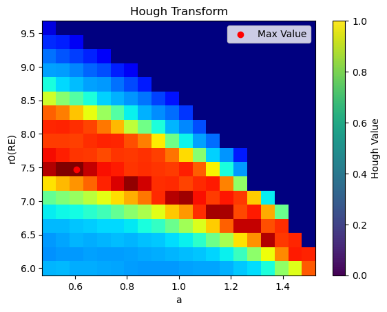
Fig. 19 Hough matrix

For each curve in the image coordinates, we calculate the intensity of the image along the curve and save its mean value in an array element. This gives us a measure of how prominent and bright this curve is in the image. We can now use this metric as a voting scheme between the curves by moving to the parameter space. Each curve and mean intensity correspond to specific initial parameters \(\alpha\) and \(r_0\). We can construct a parameter matrix with the values of the mean intensity over each curve. The visualization of this matrix in a contour plot is shown in Fig. 19. In this figure, the maximum value in parameter space is noted with the red dot. The coordinates of this point, correspond to the model parameters that return the brightest projection in the image. Moving back to image space, we can plot only the curve that correspond to these parameters, getting the best fitted Shue projection directly to the image.

The algorithm of the Hough transform is encapsulated in the hough method of the Images class:

def hough(self, r0_array, a_array):
    ### Here we set an arbitrary limit to entering the magnetopause. With the complete satellite data we can do that by using the analyser's data to determine in which region we are in and wether we should process the image.
    d_satellite = np.sqrt(self.position[0]**2+self.position[1]**2+self.position[2]**2)
    if d_satellite<7:
        return None,None,None
    # Initialize the Hough matrix
    hough = np.zeros((len(r0_array), len(a_array)))
    normalized = (self.image - np.min(self.image)) / (np.max(self.image) - np.min(self.image))
    tangent_eq_num = sp.lambdify((theta, phi, a_symb, r0_symb), self.tangent_equation(), modules='numpy')

    for i in range(len(r0_array)):
        for j in range(len(a_array)):
            Theta, Phi = Theta_grid, Phi_grid
            # Get tagent curve
            x_tangent_GSE, y_tangent_GSE, z_tangent_GSE = self.solve_tangent_GSE(r0_array[i], a_array[j], Theta, Phi, tangent_eq_num)
            x_tangent_sat , y_tangent_sat, z_tangent_sat = np.zeros((len(x_tangent_GSE))), np.zeros((len(x_tangent_GSE))), np.zeros((len(x_tangent_GSE)))
            for k in range(len(x_tangent_GSE)):
                x_tangent_sat[k], y_tangent_sat[k], z_tangent_sat[k] = self.GSE_to_Sat(x_tangent_GSE[k], y_tangent_GSE[k], z_tangent_GSE[k])
            azim_SXI, elev_SXI = self.Sat_to_SXI(x_tangent_sat, y_tangent_sat, z_tangent_sat)
            az_ind, el_ind = self.interpolate(azim_SXI, elev_SXI)
            hough[i,j] = np.mean(normalized[el_ind,az_ind])
    max_index = np.unravel_index(np.argmax(hough), hough.shape)
    return hough, r0_array[max_index[0]], a_array[max_index[1]]