
Previous work: Fitting methods#
When attempting to extract three-dimensional information from a two- dimensional image, one must make a set of assumptions to account for this loss of information. In this end, three notable techniques have been proposed to reconstruct the magnetopause using soft X-ray imaging.
The first is the Boundary Fitting Approach (BFA), introduced by [Jorgensen et al., 2019]. This method assumes parametrized forms for the magnetopause, and corresponding X-ray emissivity distribution based on MHD simulations. They then vary the parameters and generate a set of simulated images. These images are compared and fitted to the synthetic observed image, and the best-fit parameters define the optimal parameters for the reconstruction of the 3D magnetopause. BFA is effective even during rapid solar wind changes but requires a good initial guess. It also has a strong dependency on the simulation itself, since in the real-world scenario, it must fit the SXI images using only the simulation generated predictions. Further work has been done on advancing this method, leading to more sophisticated parametrization and models, such as the CMEM model [Wharton et al., 2025].
The second method, proposed by [Collier and Connor, 2018], is the Tangent Direction Approach (TDA). It is based on the hypothesis that the peak X-ray intensity corresponds to the tangent line-of-sight to the magnetopause. By analyzing this intensity variation and comparing two images from nearby viewing points, the tangent point can be located. This can be thought of as a minimalistic tomographic technique, where a static magnetopause during the two images is necessary to derive meaningful information. This may be applied to cases of steady solar wind conditions, but cannot provide dynamic information, since the integration time of a single image is in the order of 10 minutes.
Finally, [Sun et al., 2020] proposed a fitting scheme, based on the same hypothesis as Tangent Fitting Approach (TFA) - the tangent hypothesis. In her paper, she assumes that the maximum intensity arc of the integrated image corresponds to the tangent direction of the magnetopause surface. She also verifies this hypothesis for the case of an observer at infinity (parallel integration of LOS of an MHD emissivity cube. A secondary assumption is also necessary to transfer from a two-dimensional curve to a three-dimensional surface. Here it is proposed to assume the shape of the magnetopause by fitting empirical magnetopause models to the maximum intensity curve of the image.
The tangent hypothesis was re-examined more thoroughly by [Samsonov et al., 2022]. Multiple metrics for the definition of the magnetopause from the X-ray emission were tested and compared to the projection of magnetosphere’s boundary in the 3D simulation cube. To extract this boundary from the simulation, they determine the magnetospheric region using the thresholds conditions for the thermal pressure and velocity. The response of the instrument is also taken into account, and a good agreement is found between the maximum gradient of intensity arc and the tangent direction of the magnetopause.
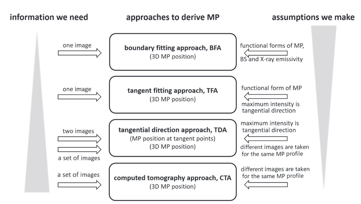
Fig. 9 Magnetopause extraction techniques and their assumptions/required input [Sun et al., 2020].#
It is evident that this method displays some key restrictions. Since the TFA calculates the tangent directions of the magnetopause, it is not applicable while the satellite is inside the magnetosphere. This POV dependency was further studied by [Read, 2024], through analyzing the validity of the tangent hypothesis in response to different viewing geometries and satellite orbits. He shows that accurate tangent fitting strongly depends on the spacecraft’s position along the orbit: only when SMILE is significantly outside the magnetopause does the peak intensity reliably trace the magnetopause tangent, while near-perigee observations fail. He also performed an interesting case study, where he generated a spherical pseudo-surface (i.e. a magnetopause proxy) to illustrate the limits of the tangent hypothesis, using a simple geometry. By applying an emissivity gradient to the pseudo-surface he demonstrated a systematic ~0.3 RE error in the tangent hypothesis caused by these gradients - highlighting that spatial emissivity variations bias tangent-based fitting. This demonstrated both the orbit-dependence of the fitting accuracy and the emissivity gradients contribution to the error. This study was performed using MHD simulated emissivity cubes, while the metrics were derived using one-point (maximum intensity) comparison to the projected surface [Read, 2024]. No fitting methods were developed or tested in these cases, leaving us with an estimation of the hypothesis error, but no concrete results on how this propagates to the final measurements.
We will attempt to understand the applicability of the tangent fitting method using the LaTeP model. To do that we need to examine its assumptions, consisting of two dependencies; first that the maximum integrated intensity coincides with the tangent direction of the magnetopause surface, and second that the empirical model we have chosen is a good description of its shape. We can then develop a methodology that will allow us to extract the empirical model parameters, from each SXI image, and reconstruct the 3D magnetopause. We will address these issues in the following chapters.