Earth’s Magnetopause

For a more precise definition of the magnetopause we shall first take a look at the properties of plasma discontinuities. Discontinuities separate plasma regions with distinct physical properties, which may change abruptly across the boundary. These changes are not arbitrary; the fields and plasma parameters must satisfy specific conditions derived from the conservation laws of mass, momentum, and energy. A standard approach to determine these boundary conditions is to integrate the MHD conservation equations across the discontinuity. This yields the Rankine-Hugoniot jump conditions, which relate quantities on both sides of the boundary.

Among the results, it follows that the normal component of the magnetic field is continuous across any discontinuity, and that the normal mass flux remains constant. Depending on how the remaining field and plasma components behave, three main classes of MHD discontinuities can be identified: tangential, rotational, and shock discontinuities. The magnetopause is most often treated as a tangential discontinuity, characterized by a discontinuous change in the tangential magnetic field and plasma flow, but continuous normal components. There is no mass or magnetic flux transfer across the boundary, and the Rankine-Hugoniot jump conditions simplify to:

\[\begin{split} [v_n] &= 0\quad \text{(zero normal flow)}\\ [B_n] &= 0 \quad \text{(zero normal magnetic field)}\\ [\rho v_n] &= 0\quad \text{(mass flux continuity)} \\ \left[ p + \frac{B^2}{2\mu_0} \right] &= 0 \quad \text{(continuity of the total pressure)}\\ [\rho] &\neq 0 \quad \text{(density can change)} \\ [\mathbf{v}_t] &\neq 0 \quad \text{(tangential velocity can change)} \\ [\mathbf{B}_t] &\neq 0 \quad \text{(tangential magnetic field can change)} \end{split}\]

We can visualize these jumps, through the typical changes in plasma moments across a tangential discontinuity, in \autoref{fig:tangential_discontinuity}. The continuity of the total pressure across the discontinuity defines a surface of total pressure balance between the two contacting plasmas with no mass or magnetic flux crossing the discontinuity from either side, while all other quantities can experience arbitrary changes. This implies, that as a tangential discontinuity the magnetopause is a surface of total pressure equilibrium between the solar wind magnetosheath plasma and the geomagnetic field confined in the magnetosphere. The \ac{IMF} is quite weak near the Earth and the magnetopsheric plasma thermal and dynamic pressures can be neglected compared with the pressure of the geomagnetic field. We can therefore, request pressure equilibrium between the dynamic pressure of the solar wind and magnetic pressure of the magnetosphere, as a first approximation.

(1)\[ 2 \mu_0 \kappa n_{sw} m_i \left( \frac{\nabla S_{mp}}{|\nabla S_{mp}|} \cdot \mathbf{v}_{sw} \right)^2 = \left( \frac{\nabla S_{mp}}{|\nabla S_{mp}|} \times \mathbf{B} \right)^2 \]

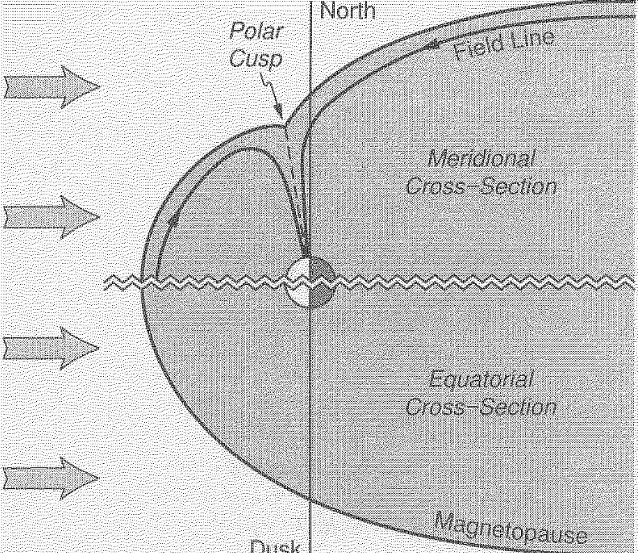
Fig. 3 Numerical solution for magnetopause.

Equation (1) contains the complicated structure of the magnetospheric magnetic field, as well as the three-dimensional derivatives of the unknown magnetopause surface \(S_{mp}\). It is a second-order three-dimensional nonlinear partial differential equation, and is therefore solvable only with numerical methods. Solving for the surface in the meridional plane, we get no continuous solution connecting the dayside magnetopause to the nightside magnetopause, while in the equatorial plane the magnetopause is a smooth curve extending from the dayside into an open tail. This point of discontinuity is defined as the polar cusp. A schematic of this solution can be found in Fig. 3.

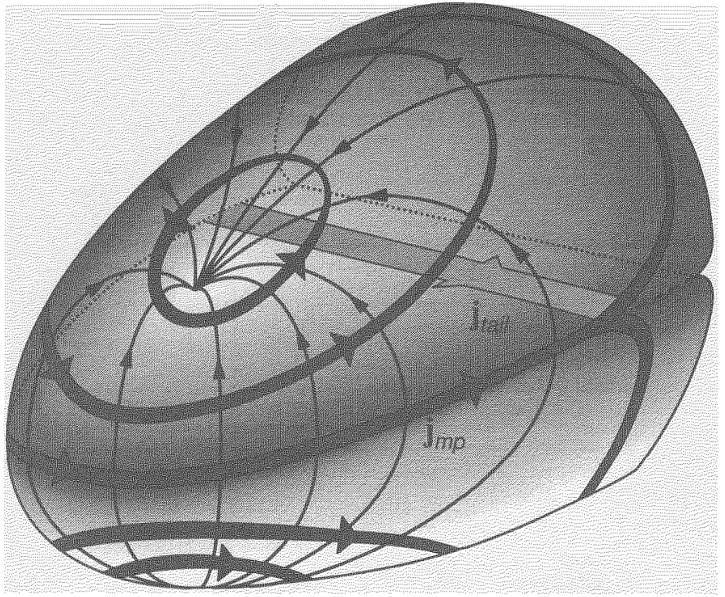
Fig. 4 Magnetopause current sheet.

The ions and electrons that are reflected at the boundary, perform partial gyro-orbits within the magnetospheric field. Their opposite gyration directions generate a net current localized near the magnetopause, with a thickness on the order of the ion gyroradius. This diamagnetic current enhances the internal magnetic field and cancels the external one, maintaining pressure balance across the boundary. We refer to this as the magnetopause current sheet, and a schematic of its structure is shown in Fig. 4. [Baumjohann and Treumann, 2006]